pytrnsys_process.api package

Module contents

pytrnsys_process package for processing TRNSYS simulation results.

This package provides tools and utilities for analyzing and processing TRNSYS simulation output data.

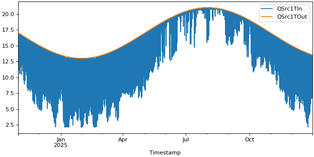
pytrnsys_process.api.line_plot(df: DataFrame, columns: list[str], use_legend: bool = True, size: tuple[float, float] = (7.8, 3.9), **kwargs: Any) → tuple[Figure, Axes]

Create a line plot using the provided DataFrame columns.

Parameters:

• df (pandas.DataFrame) – the dataframe to plot

• columns (list of str) – names of columns to plot

• use_legend (bool, default 'True') – whether to show the legend or not

• size (tuple of (float, float)) – size of the figure (width, height)

• **kwargs – Additional keyword arguments are documented in pandas.DataFrame.plot().

Return type:

tuple of (matplotlib.figure.Figure, matplotlib.axes.Axes)

Examples

>>> api.line_plot(simulation.hourly, ["QSrc1TIn", "QSrc1TOut"])

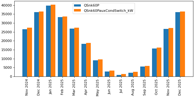
pytrnsys_process.api.bar_chart(df: DataFrame, columns: list[str], use_legend: bool = True, size: tuple[float, float] = (7.8, 3.9), **kwargs: Any) → tuple[Figure, Axes]

Create a bar chart with multiple columns displayed as grouped bars. The **kwargs are currently not passed on.

Parameters:

• df (pandas.DataFrame) – the dataframe to plot

• columns (list of str) – names of columns to plot

• use_legend (bool, default 'True') – whether to show the legend or not

• size (tuple of (float, float)) – size of the figure (width, height)

• **kwargs – Additional keyword arguments to pass on to pandas.DataFrame.plot().

Return type:

tuple of (matplotlib.figure.Figure, matplotlib.axes.Axes)

Examples

>>> api.bar_chart(simulation.monthly, ["QSnk60P","QSnk60PauxCondSwitch_kW"])

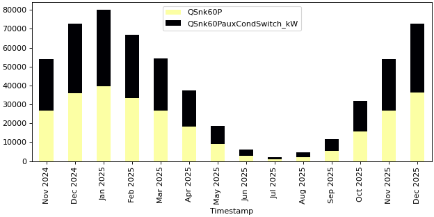
pytrnsys_process.api.stacked_bar_chart(df: DataFrame, columns: list[str], use_legend: bool = True, size: tuple[float, float] = (7.8, 3.9), **kwargs: Any) → tuple[Figure, Axes]

Bar chart with stacked bars

Parameters:

• df (pandas.DataFrame) – the dataframe to plot

• columns (list of str) – names of columns to plot

• use_legend (bool, default 'True') – whether to show the legend or not

• size (tuple of (float, float)) – size of the figure (width, height)

• **kwargs – Additional keyword arguments to pass on to pandas.DataFrame.plot().

Return type:

tuple of (matplotlib.figure.Figure, matplotlib.axes.Axes)

Examples

>>> api.stacked_bar_chart(simulation.monthly, ["QSnk60P","QSnk60PauxCondSwitch_kW"])

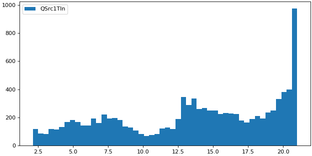
pytrnsys_process.api.histogram(df: DataFrame, columns: list[str], use_legend: bool = True, size: tuple[float, float] = (7.8, 3.9), bins: int = 50, **kwargs: Any) → tuple[Figure, Axes]

Create a histogram from the given DataFrame columns.

Parameters:

• df (pandas.DataFrame) – the dataframe to plot

• columns (list of str) – names of columns to plot

• use_legend (bool, default 'True') – whether to show the legend or not

• size (tuple of (float, float)) – size of the figure (width, height)

• bins (int) – number of histogram bins to be used

• **kwargs – Additional keyword arguments to pass on to pandas.DataFrame.plot().

Return type:

tuple of (matplotlib.figure.Figure, matplotlib.axes.Axes)

Examples

>>> api.histogram(simulation.hourly, ["QSrc1TIn"], ylabel="")

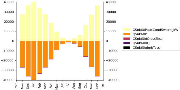
pytrnsys_process.api.energy_balance(df: DataFrame, q_in_columns: list[str], q_out_columns: list[str], q_imb_column: str | None = None, use_legend: bool = True, size: tuple[float, float] = (7.8, 3.9), **kwargs: Any) → tuple[Figure, Axes]

Create a stacked bar chart showing energy balance with inputs, outputs and imbalance. This function creates an energy balance visualization where:

• Input energies are shown as positive values

• Output energies are shown as negative values

• Energy imbalance is either provided or calculated as (sum of inputs + sum of outputs)

Parameters:

• df (pandas.DataFrame) – the dataframe to plot

• q_in_columns (list of str) – column names representing energy inputs

• q_out_columns (list of str) – column names representing energy outputs

• q_imb_column (list of str, optional) – column name containing pre-calculated energy imbalance

• use_legend (bool, default 'True') – whether to show the legend or not

• size (tuple of (float, float)) – size of the figure (width, height)

• **kwargs – Additional keyword arguments to pass on to pandas.DataFrame.plot().

Return type:

tuple of (matplotlib.figure.Figure, matplotlib.axes.Axes)

Examples

>>> api.energy_balance(
>>> simulation.monthly,
>>> q_in_columns=["QSnk60PauxCondSwitch_kW"],
>>> q_out_columns=["QSnk60P", "QSnk60dQlossTess", "QSnk60dQ"],
>>> q_imb_column="QSnk60qImbTess",
>>> xlabel=""
>>> )

pytrnsys_process.api.energy_balance_with_lines(df: DataFrame, q_in_columns: list[str], q_out_columns: list[str], line_columns: list[str] | None = None, q_imb_column: str | None = None, use_legend: bool = True, size: tuple[float, float] = (7.8, 3.9), **kwargs: Any) → tuple[Figure, Axes, Axes]

Create a stacked bar chart showing energy balance with inputs, outputs and imbalance. On top of which one or more lines will be plotted.

This function creates an energy balance visualization where:

• Input energies are shown as positive values

• Output energies are shown as negative values

• Energy imbalance is either provided or calculated as (sum of inputs + sum of outputs)

Parameters:

• df (pandas.DataFrame) – the dataframe to plot

• q_in_columns (list of str) – column names representing energy inputs

• q_out_columns (list of str) – column names representing energy outputs

• q_imb_column (list of str, optional) – column name containing pre-calculated energy imbalance

• line_columns (list of str) – column names that should be plotted as line on top of the energy balance.

• use_legend (bool, default 'True') – whether to show the legend or not

• size (tuple of (float, float)) – size of the figure (width, height)

• energy_balance_ylabel (str) – y-axis label for the energy balance.

• line_ylabel (str) – y-axis label for the lines.

• **kwargs – Additional keyword arguments to pass on to pandas.DataFrame.plot().

Return type:

tuple of (matplotlib.figure.Figure, matplotlib.axes.Axes)

Examples

>>> api.energy_balance_with_lines(
>>> simulation.monthly,
>>> q_in_columns=["QSnk60PauxCondSwitch_kW"],
>>> q_out_columns=["QSnk60P", "QSnk60dQlossTess", "QSnk60dQ"],
>>> q_imb_column="QSnk60qImbTess",
>>> xlabel=""
>>> )

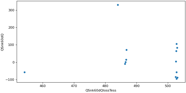
pytrnsys_process.api.scatter_plot(df: DataFrame, x_column: str, y_column: str, use_legend: bool = True, size: tuple[float, float] = (7.8, 3.9), **kwargs: Any) → tuple[Figure, Axes]

Create a scatter plot to show numerical relationships between x and y variables.

Note

Use color and not cmap!

See: https://pandas.pydata.org/pandas-docs/stable/reference/api/pandas.DataFrame.plot.scatter.html

Parameters:

• df (pandas.DataFrame) – the dataframe to plot

• x_column (str) – coloumn name for x-axis values

• y_column (str) – coloumn name for y-axis values

use_legend: bool, default ‘True’

whether to show the legend or not

size: tuple of (float, float)

size of the figure (width, height)

**kwargs :

Additional keyword arguments to pass on to pandas.DataFrame.plot.scatter().

Return type:

tuple of (matplotlib.figure.Figure, matplotlib.axes.Axes)

Examples

Simple scatter plot

>>> api.scatter_plot(
...     simulation.monthly, x_column="QSnk60dQlossTess", y_column="QSnk60dQ"
... )

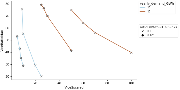
pytrnsys_process.api.scalar_compare_plot(df: DataFrame, x_column: str, y_column: str, group_by_color: str | None = None, group_by_marker: str | None = None, use_legend: bool = True, size: tuple[float, float] = (7.8, 3.9), scatter_kwargs: dict[str, Any] | None = None, line_kwargs: dict[str, Any] | None = None, **kwargs: Any) → tuple[Figure, Axes]

Create a scalar comparison plot with up to two grouping variables. This visualization allows simultaneous analysis of:

• Numerical relationships between x and y variables

• Categorical grouping through color encoding

• Secondary categorical grouping through marker styles

Note

To change the figure properties a separation is included. scatter_kwargs are used to change the markers. line_kwargs are used to change the lines.

See: - markers: https://matplotlib.org/stable/api/_as_gen/matplotlib.axes.Axes.scatter.html - lines: https://matplotlib.org/stable/api/_as_gen/matplotlib.axes.Axes.plot.html

Parameters:

• df (pandas.DataFrame) – the dataframe to plot

• x_column (str) – column name for x-axis values

• y_column (str) – column name for y-axis values

• group_by_color (str, optional) – column name for color grouping

• group_by_marker (str, optional) – column name for marker style grouping

• use_legend (bool, default 'True') – whether to show the legend or not

• size (tuple of (float, float)) – size of the figure (width, height)

• line_kwargs – Additional keyword arguments to pass on to matplotlib.axes.Axes.plot().

• scatter_kwargs – Additional keyword arguments to pass on to matplotlib.axes.Axes.scatter().

• **kwargs – Should never be used! Use ‘line_kwargs’ or ‘scatter_kwargs’ instead.

Return type:

tuple of (matplotlib.figure.Figure, matplotlib.axes.Axes)

Examples

Compare plot

>>> api.scalar_compare_plot(
...     comparison_data,
...     x_column="VIceSscaled",
...     y_column="VIceRatioMax",
...     group_by_color="yearly_demand_GWh",
...     group_by_marker="ratioDHWtoSH_allSinks",
... )

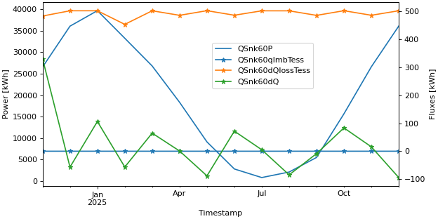
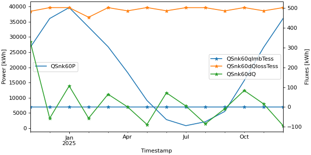
pytrnsys_process.api.get_figure_with_twin_x_axis() → tuple[Figure, Axes, Axes]

Used to make figures with different y axes on the left and right. To create such a figure, pass the lax to one plotting method and pass the rax to another.

Warning

Be careful when combining plots. MatPlotLib will not complain when you provide incompatible x-axes. An example: combining a time-series with dates with a histogram with temperatures. In this case, the histogram will disappear without any feedback.

Note

The legend of a twin_x plot is a special case: To have all entries into a single plot, use fig.legend https://matplotlib.org/stable/api/_as_gen/matplotlib.figure.Figure.legend.html

To instead have two separate legends, one for each y-axis, use lax.legend and rax.legend. https://matplotlib.org/stable/api/_as_gen/matplotlib.axes.Axes.legend.html

Returns:

• fig – Figure object

• lax – Axis object for the data on the left y-axis.

• rax – Axis object for the data on the right y-axis.

Examples

Twin axis plot with a single legend

>>> fig, lax, rax = api.get_figure_with_twin_x_axis()
>>> api.line_plot(simulation.monthly, ["QSnk60P",], ylabel="Power [kWh]", use_legend=False, fig=fig, ax=lax)
>>> api.line_plot(simulation.monthly, ["QSnk60qImbTess", "QSnk60dQlossTess", "QSnk60dQ"], marker="*",
...     ylabel="Fluxes [kWh]", use_legend=False, fig=fig, ax=rax)
>>> fig.legend(loc="center", bbox_to_anchor=(0.6, 0.7))

Twin axis plot with two legends

>>> fig, lax, rax = api.get_figure_with_twin_x_axis()
>>> api.line_plot(simulation.monthly, ["QSnk60P",], ylabel="Power [kWh]", use_legend=False, fig=fig, ax=lax)
>>> api.line_plot(simulation.monthly, ["QSnk60qImbTess", "QSnk60dQlossTess", "QSnk60dQ"], marker="*",
...     ylabel="Fluxes [kWh]", use_legend=False, fig=fig, ax=rax)
>>> lax.legend(loc="center left")
>>> rax.legend(loc="center right")

pytrnsys_process.api.process_whole_result_set_parallel(results_folder: Path, processing_scenario: Callable[[Simulation], None] | Sequence[Callable[[Simulation], None]], max_workers: int | None = None) → SimulationsData

Process all simulation folders in a results directory in parallel.

Uses a ProcessPoolExecutor to process multiple simulations concurrently, applying the provided processing step/scenario to each simulation.

Using the default settings your structure should look like this:

results_folder

├─ sim-1

├─ sim-2

├─ sim-3

├─ temp

├─ your-printer-files.prt

Parameters:

• pathlib.Path (results_folder) – Path to the directory containing simulation folders. Each subfolder should contain a temp folder containing valid simulation data files.

• processing_scenario (collections.abc.Callable or collections.abc.Sequence of collections.abc.Callable) – They should containd the processing logic for a simulation. Each callable should take a Simulation object as its only parameter and modify it in place.

• int (max_workers) – Maximum number of worker processes to use. If None, defaults to the number of processors on the machine.

• None (default) – Maximum number of worker processes to use. If None, defaults to the number of processors on the machine.

Returns:

SimulationsData –

• monthly: Dict mapping simulation names to monthly DataFrame results

• hourly: Dict mapping simulation names to hourly DataFrame results

• scalar: DataFrame containing scalar/deck values from all simulations

Return type:

pytrnsys_process.api.SimulationsData

Raises:

• ValueError – If results_folder doesn’t exist or is not a directory:

• Exception – Individual simulation failures are logged but not re-raised:

Example

>>> import pathlib as _pl
>>> from pytrnsys_process import api
...
>>> def processing_step_1(sim):
...     # Process simulation data
...     pass
>>> def processing_step_2(sim):
...     # Process simulation data
...     pass
>>> results = api.process_whole_result_set_parallel(
...     _pl.Path("path/to/results"),
...     [processing_step_1, processing_step_2]
... )

pytrnsys_process.api.process_single_simulation(sim_folder: Path, processing_scenario: Callable[[Simulation], None] | Sequence[Callable[[Simulation], None]]) → Simulation

Process a single simulation folder using the provided processing step/scenario.

Parameters:

• sim_folder (pathlib.Path) – Path to the simulation folder to process

• processing_scenario (collections.abc.Callable or collections.abc.Sequence of collections.abc.Callable) – They should contain the processing logic for a simulation. Each callable should take a Simulation object as its only parameter and modify it in place.

Returns:

Simulation

Return type:

pytrnsys_process.api.Simulation

Example

>>> import pathlib as _pl
>>> from pytrnsys_process import api
...
>>> def processing_step_1(sim: api.Simulation):
...     # Process simulation data
...     pass
>>> results = api.process_single_simulation(
...     _pl.Path("path/to/simulation"),
...     processing_step_1
... )

pytrnsys_process.api.process_whole_result_set(results_folder: Path, processing_scenario: Callable[[Simulation], None] | Sequence[Callable[[Simulation], None]]) → SimulationsData

Process all simulation folders in a results directory sequentially.

Processes each simulation folder found in the results directory one at a time, applying the provided processing step/scenario to each simulation.

Using the default settings your structure should look like this:

results_folder

├─ sim-1

├─ sim-2

├─ sim-3

├─ temp

├─ your-printer-files.prt

Parameters:

• pathlib.Path (results_folder) – Path to the directory containing simulation folders. Each subfolder should contain a temp folder containing valid simulation data files.

• processing_scenario (collections.abc.Callable or collections.abc.Sequence of collections.abc.Callable) – They should containd the processing logic for a simulation. Each callable should take a Simulation object as its only parameter and modify it in place.

Returns:

SimulationsData –

• monthly: Dict mapping simulation names to monthly DataFrame results

• hourly: Dict mapping simulation names to hourly DataFrame results

• scalar: DataFrame containing scalar/deck values from all simulations

Return type:

pytrnsys_process.api.SimulationsData

Raises:

• ValueError – If results_folder doesn’t exist or is not a directory:

• Exception – Individual simulation failures are logged but not re-raised:

Example

>>> import pathlib as _pl
>>> from pytrnsys_process import api
...
>>> def processing_step_1(sim):
...     # Process simulation data
...     pass
>>> def processing_step_2(sim):
...     # Process simulation data
...     pass
>>> results = api.process_whole_result_set(
...     _pl.Path("path/to/results"),
...     [processing_step_1, processing_step_2]
... )

pytrnsys_process.api.do_comparison(comparison_scenario: Callable[[SimulationsData], None] | Sequence[Callable[[SimulationsData], None]], simulations_data: SimulationsData | None = None, results_folder: Path | None = None) → SimulationsData

Execute comparison scenarios on processed simulation results.

Parameters:

• comparison_scenario (collections.abc.Callable or collections.abc.Sequence of collections.abc.Callable) – They should containd the comparison logic. Each callable should take a SimulationsData object as its only parameter and modify it in place.

• simulations_data (SimulationsData, optional) – SimulationsData object containing the processed simulations data to be compared.

• results_folder (pathlib.Path, optional) – Path to the directory containing simulation results. Used if simulations_data is not provided.

Returns:

SimulationsData

Return type:

pytrnsys_process.api.SimulationsData

Example

>>> from pytrnsys_process import api
...
>>> def comparison_step(simulations_data: ds.SimulationsData):
...     # Compare simulation results
...     pass
...
>>> api.do_comparison(comparison_step, simulations_data=processed_results)

pytrnsys_process.api.export_plots_in_configured_formats(fig: Figure, path_to_directory: str, plot_name: str, plots_folder_name: str = 'plots') → None

Save a matplotlib figure in multiple formats and sizes.

Saves the figure in all configured formats (png, pdf, emf) and sizes (A4, A4_HALF) as specified in the plot settings (api.settings.plot). For EMF format, the figure is first saved as SVG and then converted using Inkscape.

Parameters:

• fig – The matplotlib Figure object to save.

• path_to_directory – Directory path where the plots should be saved.

• plot_name – Base name for the plot file (will be appended with size and format).

• plots_folder_name – leave empty if you don’t want to save in a new folder

Note

• Creates a ‘plots’ subdirectory if it doesn’t exist

• For EMF files, requires Inkscape to be installed at the configured path

• File naming format: {plot_name}-{size_name}.{format}

Example

>>> from pytrnsys_process import api, data_structures
>>> def processing_of_monthly_data(simulation: data_structures.Simulation):
>>>     monthly_df = simulation.monthly
>>>     columns_to_plot = ["QSnk60P", "QSnk60PauxCondSwitch_kW"]
>>>     fig, ax = api.bar_chart(monthly_df, columns_to_plot)
>>>
>>>     # Save the plot in multiple formats
>>>     api.export_plots_in_configured_formats(fig, simulation.path, "monthly-bar-chart")
>>>     # Creates files like:
>>>     #   results/simulation1/plots/monthly-bar-chart-A4.png
>>>     #   results/simulation1/plots/monthly-bar-chart-A4.pdf
>>>     #   results/simulation1/plots/monthly-bar-chart-A4.emf
>>>     #   results/simulation1/plots/monthly-bar-chart-A4_HALF.png
>>>     #   etc.

class pytrnsys_process.api.Defaults(*values)

Bases: Enum

Default settings for different use cases

DEFAULT = Settings(plot=Plot(file_formats=['.png', '.pdf', '.emf'], figure_sizes={'A4': (7.8, 3.9), 'A4_HALF': (3.8, 3.9)}, inkscape_path='C://Program Files//Inkscape//bin//inkscape.exe', date_format='%b %Y', label_font_size=10, legend_font_size=8, title_font_size=12, markers=['x', 'o', '^', 'D', 'v', '<', '>', 'p', '*', 's']), reader=Reader(folder_name_for_printer_files='temp', read_step_files=False, read_deck_files=True, force_reread_prt=False, starting_year=2024))

class pytrnsys_process.api.Simulation(path: str, monthly: DataFrame, hourly: DataFrame, step: DataFrame, scalar: DataFrame)

Bases: object

Class representing a TRNSYS simulation with its associated data.

This class holds the simulation data organized in different time resolutions (monthly, hourly, timestep) along with the path to the simulation files.

path

Path to the simulation folder containing the input files

Type:

str

monthly

Monthly aggregated simulation data. Each column represents a different variable and each row represents a month.

Type:

pandas.DataFrame

hourly

Hourly simulation data. Each column represents a different variable and each row represents an hour.

Type:

pandas.DataFrame

step

Simulation data at the smallest timestep resolution. Each column represents a different variable and each row represents a timestep.

Type:

pandas.DataFrame

__init__(path: str, monthly: DataFrame, hourly: DataFrame, step: DataFrame, scalar: DataFrame) → None

path: str

monthly: DataFrame

hourly: DataFrame

step: DataFrame

scalar: DataFrame

class pytrnsys_process.api.SimulationsData(simulations: dict[str, ~pytrnsys_process.process.data_structures.Simulation] = <factory>, scalar: ~pandas.core.frame.DataFrame = <factory>, path_to_simulations: str = <factory>)

Bases: object

Class representing a result set

Used to do comparisons plots across different simulations

simulations

Can be accessed using the simulations names as keys. Example: simulations['sim_001']

Type:

dict of {str, Simulation}

scalar

Contains all deck constant deck values from all simulations. This is also the place to store your calculations for plotting.

Type:

pandas.DataFrame

path_to_simulations

The path to your results folder

Type:

str

__init__(simulations: dict[str, ~pytrnsys_process.process.data_structures.Simulation] = <factory>, scalar: ~pandas.core.frame.DataFrame = <factory>, path_to_simulations: str = <factory>) → None

simulations: dict[str, Simulation]

scalar: DataFrame

path_to_simulations: str

path_to_simulations_original: str

pytrnsys_process.api.load_simulations_data_from_pickle(path: ~pathlib.Path, logger: ~logging.Logger = <Logger default_pytrnsys_process (WARNING)>) → SimulationsData

Load SimulationsData from a pickle file.

This function loads a previously saved SimulationsData object from a pickle file.

Parameters:

• path (pathlib.Path) – To the pickle file to load

• logger (logging.Logger, optional) – Logger object that will log any messages, warnings, and/or errors

Returns:

SimulationsData – Reconstructed SimulationsData object

Return type:

pytrnsys_processing.data_structures.SimulationsData

Raises:

• OSError – If there’s an error reading the file:

• pickle.UnpicklingError – If the file is corrupted or invalid:

pytrnsys_process.api.load_simulation_from_pickle(path: ~pathlib.Path, logger: ~logging.Logger = <Logger default_pytrnsys_process (WARNING)>) → Simulation

Load a Simulation object from a pickle file.

This function loads a previously saved Simulation object from a pickle file.

Parameters:

• path (pathlib.Path) – To the pickle file to load

• logger (logging.Logger, optional) – Logger object that will log any messages, warnings, and/or errors

Returns:

Simulation – Reconstructed Simulation object

Return type:

pytrnsys_processing.data_structures.Simulation

Raises:

• OSError – If there’s an error reading the file:

• pickle.UnpicklingError – If the file is corrupted or invalid:

pytrnsys_process.api.get_date_time_axis_locator_and_formatter(data_frequency: Literal['step', 'hourly', 'monthly']) → Tuple[AutoDateLocator, ConciseDateFormatter]

Method to prepare an axis locator and a date time formattter to adjust the date time formatting. Can be used as follows: ax.xaxis.set_major_formatter(formatter) ax.xaxis.set_major_locator(date_locator)

Parameters:

data_frequency (str) – Size of the timestep. This can be ‘step’, ‘hourly’, and ‘monthly’.

pytrnsys_process.api.get_frequency_of_data(df: DataFrame) → Literal['step', 'hourly', 'monthly']

Method to identify the timestep size of the give dataframe. Can return ‘step’, ‘hourly’, and ‘monthly’.

pytrnsys_process.api.format_date_time_twin_axis(lax: Axes, rax: Axes, data_frequency: Literal['step', 'hourly', 'monthly'])

Method to update dateTime formatting for twin axes.

Parameters:

• lax (_plt.Axes) – left-axis handle

• rax (_plt.Axes) – right-axis handle

• data_frequency (str) – Size of the timestep. This can be ‘step’, ‘hourly’, and ‘monthly’.