Comparison

This tutorial will guide you to creating your own comparison plots. For a more in-depth view, please refer to the How Tos and the API docs pytrnsys_process.api

Required Imports

First, let’s add the required imports to the top of the script.

import pathlib as _pl

from pytrnsys_process import api

Preparation

First, you will need to download the example data.

Extract the data into a project folder you will use for this tutorial. You should end up with a folder structure looking like this.

root

├─ example_data

├─ tutorials

├─ tutorial_comparison.py

For the rest of this tutorial, you should work in the last file: “tutorial_comparison.py”

Defining comparison steps

This comparison step will loop through all simulations. It will use the hourly and monthly dataframes to do calculations. The results will be stored in the scalar dataframe that all simulations share. At the end we will return the modified pytrnsys_process.api.SimulationsData object. Reason for this is mentioned in the next step.

def do_calc(simulations_data: api.SimulationsData):

    for sim_name, sim in simulations_data.simulations.items():

        hourly_data = sim.hourly
        max_ice_ratio = hourly_data["VIceRatio"].max()
        simulations_data.scalar.loc[sim_name, "VIceRatioMax"] = max_ice_ratio

        demand_columns = [
            "qSysOut_QSnk131Demand",
            "qSysOut_QSnk183Demand",
            "qSysOut_QSnk191Demand",
            "qSysOut_QSnk225Demand",
            "qSysOut_QSnk243Demand",
            "qSysOut_QSnk266Demand",
            "qSysOut_QSnk322Demand",
            "qSysOut_QSnk335Demand",
            "qSysOut_QSnk358Demand",
            "qSysOut_QSnk417Demand",
            "qSysOut_QSnk448Demand",
            "qSysOut_QSnk469Demand",
            "qSysOut_QSnk488Demand",
            "qSysOut_QSnk524Demand",
            "qSysOut_QSnk539Demand",
            "qSysOut_QSnk558Demand",
            "qSysOut_QSnk579Demand",
            "qSysOut_QSnk60Demand",
            "qSysOut_QSnk85Demand",
        ]

        # Unit conversion factor: kWh to GWh
        kwh_to_gwh = 1e-6

        # Process monthly data
        monthly_df = sim.monthly
        monthly_df["total_demand_GWh"] = (
            monthly_df[demand_columns].sum(axis=1) * kwh_to_gwh
        )

        # Calculate yearly total (excluding first 2 months)
        yearly_total = int(monthly_df["total_demand_GWh"].iloc[2::].sum())
        simulations_data.scalar.loc[sim_name, "yearly_demand_GWh"] = (
            yearly_total
        )
    return simulations_data

Chain multiple comparison steps

By chaining comparison steps together, we ensure that if a dependent step fails, the entire process fails. In this step, we call the previously defined step to validate our data before generating plots. This way, if an error occurs during the calculation, we avoid plotting incorrect data.

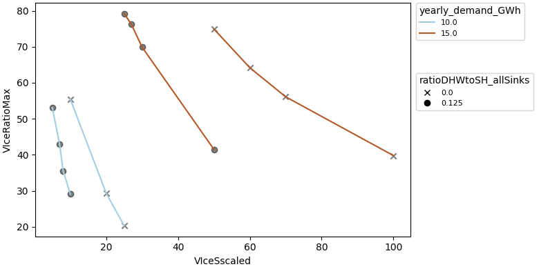
def plot_comparison(simulations_data: api.SimulationsData):
    simulations_data = do_calc(simulations_data)

    fig, _ = api.scalar_compare_plot(
        simulations_data.scalar,
        "VIceSscaled",
        "VIceRatioMax",
        group_by_color="yearly_demand_GWh",
        group_by_marker="ratioDHWtoSH_allSinks",
    )

    fig.show()

Running comparison steps

There are different ways of providing data to the do_comparison function. In this tutorial we will provide the path to our result folder. For other ways see pytrnsys_process.api.do_comparison()

if __name__ == "__main__":
    path_to_sim = _pl.Path("../example_data/ice/")
    api.do_comparison([plot_comparison], results_folder=path_to_sim)